PSTAT 5A: Conditional Probability Continued & Bayes’ Theorem
Lecture 6
Today’s Learning Objectives
By the end of this lecture, you will be able to:
- Define probability and understand its basic properties
- Identify sample spaces and events
- Apply fundamental probability rules
- Calculate conditional probabilities
- Determine when events are independent
- Use Bayes’ theorem in simple applications
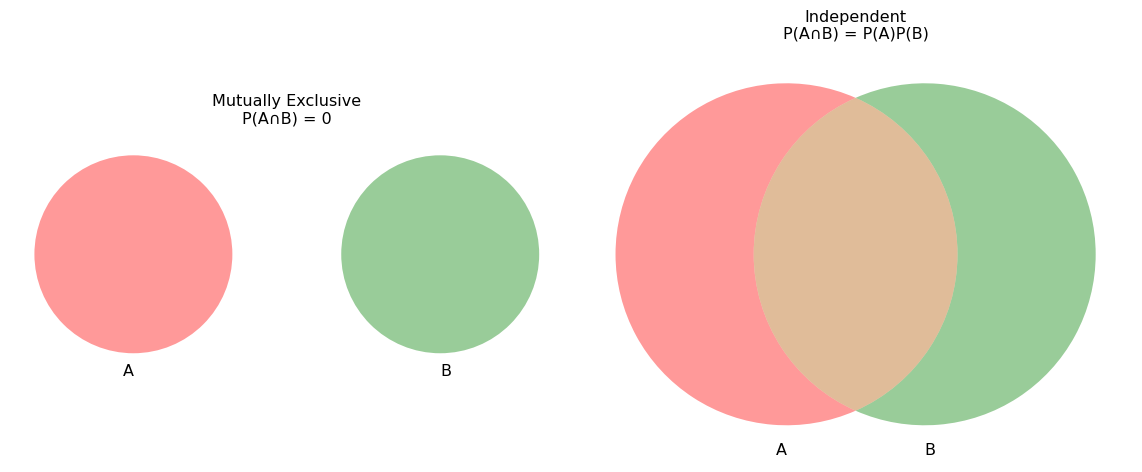
Mutually Exclusive vs. Independent
Mutually Exclusive (left): the circles A and B do not overlap, so \(P(A\cap B)=0\).
Independent (right): the circles overlap, and we’ve sized the intersection so that \(P(A\cap B)=P(A)\,P(B)\).
Mutually Exclusive vs. Independent Example
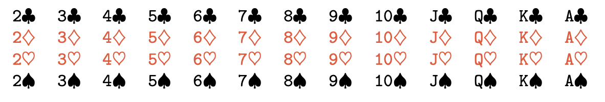
Draw a single card from a 52-card deck:
Let A={“draw an Ace”}, so P(A)=4/52.
Let B={“draw a King”}, so P(B)=4/52.
Q: What is \(P(A\cap B)\) ?
Solution. They’re disjoint (you can’t draw an Ace and a King), so \(P(A\cap B) = 0\).
But \(P(A)\,P(B) = \frac{4}{52}\times\frac{4}{52} = \frac{16}{2704} \neq 0\).
Hence, \(P(A\cap B)\neq P(A)P(B)\), so they’re not independent.
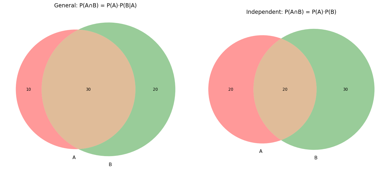
Multiplication Rule
General case: \(P(A \cap B) = P(A) \times P(B|A)\)
Independent events: \(P(A \cap B) = P(A) \times P(B)\)
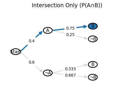
Tree Diagrams
🎯 Definition Tree diagrams help visualize sequential events and calculate probabilities.
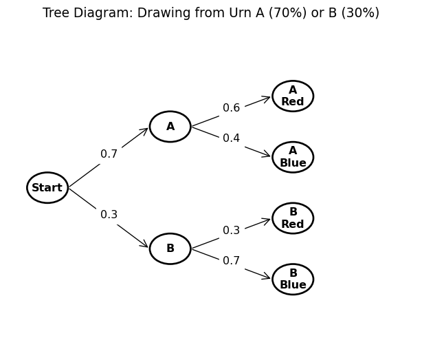
Tree Diagram Examples
Practice Problem 2
A jar contains 5 red balls and 3 blue balls. Two balls are drawn without replacement.
What’s the probability both balls are red?
What’s the probability the first is red and second is blue?
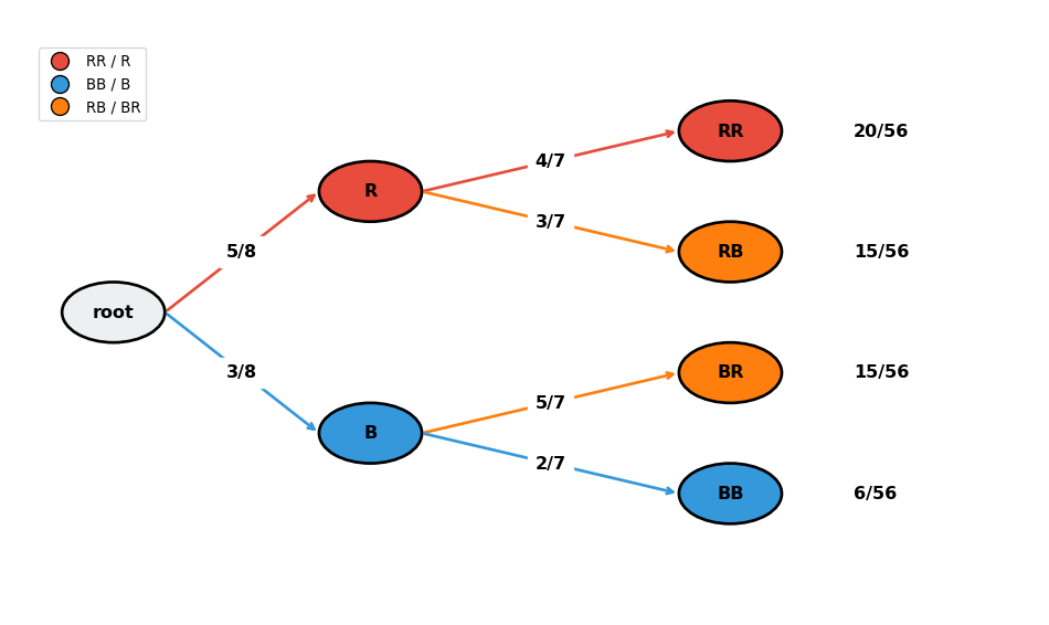
Solution.
\(P(\text{both red}) = \frac{5}{8} \times \frac{4}{7} = \frac{20}{56} = \frac{5}{14}\)
\(P(\text{red then blue}) = \frac{5}{8} \times \frac{3}{7} = \frac{15}{56}\)
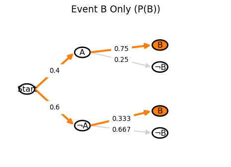
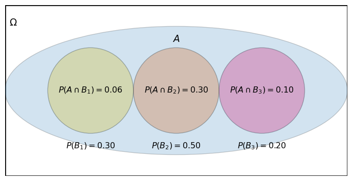
Law of Total Probability
🎯 Definition
If events \(B_1, B_2, \ldots, B_n\) form a partition of the sample space, then:
\[P(A) = P(A|B_1)P(B_1) + P(A|B_2)P(B_2) + \cdots + P(A|B_n)P(B_n)\]
Law of Total Probability Example
A factory has two machines:
Machine 1: Produces 60% of items, 5% defective
Machine 2: Produces 40% of items, 3% defective
Q: What’s the overall probability an item is defective?
Solution. \(P(\text{defective}) = P(D|M_1)P(M_1) + P(D|M_2)P(M_2)\)
\(= 0.05 \times 0.6 + 0.03 \times 0.4 = 0.03 + 0.012 = 0.042\)
Bayes’ Theorem
🎯 Definition \[P(A|B) = \frac{P(B|A) \times P(A)}{P(B)}\]
This allows us to “reverse” conditional probabilities
Named after Thomas Bayes (1701-1761)
Bayes’ Theorem Components
- \(A,B\): Events
- \(P(A|B)\): Posterior probability - what we want to find
- \(P(B|A)\): Likelihood - given \(A\), probability of observing \(B\)
- \(P(A)\): Prior probability - initial probability of \(A\)
- \(P(B)\): Marginal probability - total probability of \(B\)
Bayes’ Theorem Example
Medical test for a disease: 1
Disease affects 1% of population
Test is 95% accurate for sick people
Test is 90% accurate for healthy people
Q:If someone tests positive, what’s the probability they have the disease?
Bayes’ Theorem Solution
Let:
\(D\): Person has disease
\(T^+\): Test is positive
Given:
\(P(D) = 0.01\)
\(P(T^+|D) = 0.95\)
\(P(T^-|D^c) = 0.90\), so \(P(T^+|D^c) = 0.10\)
Solution. \(P(T^+) = P(T^+|D)P(D) + P(T^+|D^c)P(D^c)\)
\(= 0.95 \times 0.01 + 0.10 \times 0.99 = 0.1085\)
Bayes’ Theorem Solution (cont.)
\[P(D|T^+) = \frac{P(T^+|D) \times P(D)}{P(T^+)} = \frac{0.95 \times 0.01}{0.1085} \approx 0.088\]
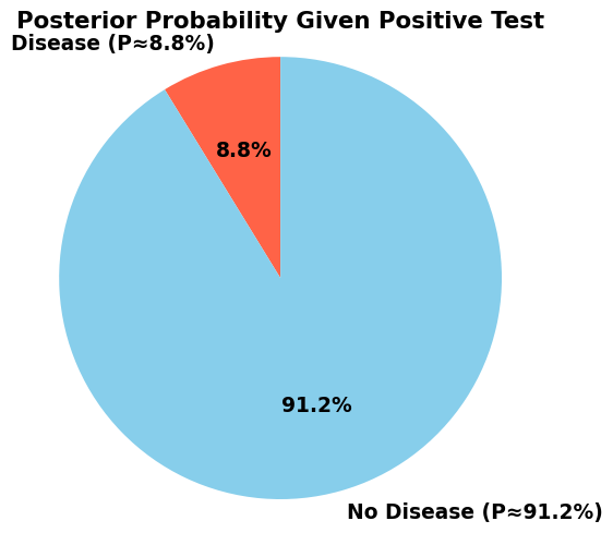
Surprising result: Even with a positive test, there’s only an 8.8% chance of having the disease!
This is due to the low base rate of the disease
Common Probability Mistakes
- Confusing \(P(A|B)\) with \(P(B|A)\)
Prosecutor’s fallacy is a specific error in interpreting conditional probabilities. Confusing
\(P(\text{Evidence}\mid\text{Innocent}) \quad\text{with}\quad P(\text{Innocent}\mid\text{Evidence})\).
Ex: OJ Simpson Case 2
Common Probability Mistakes
Assuming independence when events are dependent
Ignoring base rates (as in the medical test example)
Base rate fallacy is when you ignore or underweight the prior probability \(P(H)\) of a hypothesis, focusing only on the new evidence \(E\).
- Double counting in union calculations
Practice Problem 3
Two fair dice are rolled. Find:
- \(P(\text{sum} = 7)\)
- \(P(\text{sum} = 7 | \text{first die shows 3})\)
- Are these events independent?
Solution.
6 ways out of 36: \(P(\text{sum} = 7) = \frac{6}{36} = \frac{1}{6}\)
Given first die is 3, need second die to be 4: \(P(\text{sum} = 7 | \text{first} = 3) = \frac{1}{6}\)
Yes, they’re independent since \(P(A|B) = P(A)\)
Counting and Probability
Sometimes we need to count outcomes:
Multiplication Principle: If task 1 can be done in \(m\) ways and task 2 in \(n\) ways, both can be done in \(m \times n\) ways
Permutations: Arrangements where order matters \[P(n,r) = \frac{n!}{(n-r)!}\]
Combinations: Selections where order doesn’t matter \[C(n,r) = \binom{n}{r} = \frac{n!}{r!(n-r)!}\]
Counting Example
Q: How many ways can you arrange 5 people in a row?
Solution. This is a permutation: \(P(5,5) = 5! = 120\) ways
Q:How many ways can you choose 3 people from 5 for a committee?
Solution. This is a combination: \(C(5,3) = \binom{5}{3} = \frac{5!}{3!2!} = 10\) ways
Probability with Counting
Example: A committee of 3 people is chosen from 8 people (5 women, 3 men). What’s the probability all 3 are women?
Solution. Total ways to choose 3 from 8: \(\binom{8}{3} = 56\)
Ways to choose 3 women from 5: \(\binom{5}{3} = 10\)
Probability: \(\frac{10}{56} = \frac{5}{28}\)
Real-World Applications
Medical Diagnosis: Using Bayes’ theorem for test interpretation
Quality Control: Probability of defective items
Finance: Risk assessment and portfolio theory
Sports: Probability of wins, fantasy sports
Insurance: Calculating premiums based on risk
Key Formulas Summary
- Basic probability: \(P(A) = \frac{\text{favorable outcomes}}{\text{total outcomes}}\)
- Complement: \(P(A^c) = 1 - P(A)\)
- Addition: \(P(A \cup B) = P(A) + P(B) - P(A \cap B)\)
- Conditional: \(P(A|B) = \frac{P(A \cap B)}{P(B)}\)
- Independence: \(P(A \cap B) = P(A) \times P(B)\)
- Bayes’: \(P(A|B) = \frac{P(B|A) \times P(A)}{P(B)}\)
Problem-Solving Strategy
- Identify the sample space and events
- Determine if events are independent or mutually exclusive
- Choose the appropriate rule or formula
- Calculate step by step
- Check if your answer makes sense
Practice Problem 4
A bag contains 4 red, 3 blue, and 2 green marbles. Three marbles are drawn without replacement.
Find the probability that: a) All three are red b) No two are the same color c) At least one is blue
Practice Problem 4 Solutions
Solution.
All red: \(\frac{4}{9} \times \frac{3}{8} \times \frac{2}{7} = \frac{24}{504} = \frac{1}{21}\)
Different colors: \(\frac{4 \times 3 \times 2}{9 \times 8 \times 7} \times 3! = \frac{24 \times 6}{504} = \frac{144}{504} = \frac{2}{7}\)
At least one blue: \(1 - P(\text{no blue}) = 1 - \frac{6 \times 5 \times 4}{9 \times 8 \times 7} = 1 - \frac{120}{504} = \frac{384}{504} = \frac{16}{21}\)
Common Questions
Q1.: “Why isn’t \(P(A \cup B) = P(A) + P(B)\) always?”
A: We’d double-count outcomes in both events
Q2.: “How do I know if events are independent?”
A: Check if \(P(A|B) = P(A)\) or if \(P(A \cap B) = P(A) \times P(B)\)
Q3.: “When do I use Bayes’ theorem?”
A: When you want to “reverse” a conditional probability
Q3 note (Bayes Example)
Forward: I know my test picks up disease 95% of the time ⇒ \(P(+\mid D)=0.95\).
Reverse: I want the chance I really have the disease when the test is positive ⇒ \(P(D\mid +)\).
Looking Ahead
Next lecture:
Random Variables and Probability Distributions
Discrete vs. continuous random variables
Expected value and variance
Final Thoughts
Probability is the foundation of statistics:
Helps us quantify uncertainty
Provides tools for making decisions with incomplete information
Essential for understanding statistical inference
Practice: The key to mastering probability is working through many problems!
Questions?
Office Hours: Thursday’s 11 AM On Zoom (Link on Canvas)
Email: nmathlouthi@ucsb.edu
Next Class: Random Variables and Distributions
Resources
Footnotes
\(P(\neg D \,\wedge\, \text{Negative}) \;=\;P(\neg D)\times P(\text{Negative}\mid \neg D) \;=\;0.99\times0.90 \;=\;0.891\;(89.1\%)\)↩︎
the DNA evidence in the O. J. Simpson trial are a classic example of the prosecutor’s fallacy. Prosecutors highlighted that the chance of a random person matching the crime-scene DNA was “one in 170 million,” then implied (or let the jury infer) that Simpson therefore had a 1 in 170 million chance of being innocent.↩︎