Lab 5 Solutions: Continuous Random Variables & Confidence Intervals

PSTAT 5A - Summer Session A 2025

Getting Started - Setup Code

# Install any missing packages (will skip those already installed)
#!%pip install --quiet numpy matplotlib scipy pandas statsmodels

# Load our tools (libraries)
import numpy as np # numerical computing (arrays, random numbers, etc.)
import matplotlib.pyplot as plt # plotting library for static 2D graphs and visualizations
from scipy import stats #  statistical functions (distributions, tests, etc.)
import pandas as pd # data structures (DataFrame) and data analysis tools
import statsmodels  # statistical modeling (regression, time series, ANOVA, etc.)

# Make our graphs look nice
#!%matplotlib inline     # embed Matplotlib plots directly in the notebook
plt.style.use('seaborn-v0_8-whitegrid')  # Apply a clean whitegrid style from Seaborn

# Set random seed for reproducible results
np.random.seed(42)    # fix the random seed so results can be reproduced exactly

print("✅ All tools loaded successfully!") 

✅ All tools loaded successfully!

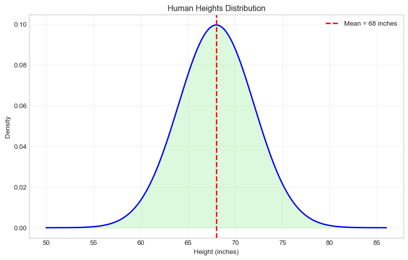
Task 1 Solution: Your First Normal Distribution

Human heights follow a normal distribution with mean = 68 inches and standard deviation = 4 inches.

# Heights distribution - SOLUTION
mean_height = 68  # SOLUTION: 68
std_height = 4    # SOLUTION: 4

heights = stats.norm(loc=mean_height, scale=std_height)

print(f"Mean height: {heights.mean()} inches")
print(f"Standard deviation: {heights.std()} inches")

Mean height: 68.0 inches
Standard deviation: 4.0 inches

# Calculate probabilities - SOLUTION

# a) What's the probability someone is taller than 72 inches (6 feet)?
prob_tall = 1 - heights.cdf(72)  # SOLUTION: 72
print(f"P(height > 72 inches) = {prob_tall:.4f}")

# b) What's the probability someone is between 64 and 72 inches?
prob_between = heights.cdf(72) - heights.cdf(64)  # SOLUTION: 72, 64
print(f"P(64 < height < 72) = {prob_between:.4f}")

# c) What height is at the 90th percentile? (90% of people are shorter)
height_90th = heights.ppf(0.90)  # SOLUTION: 0.90
print(f"90th percentile height: {height_90th:.2f} inches")

P(height > 72 inches) = 0.1587
P(64 < height < 72) = 0.6827
90th percentile height: 73.13 inches

# Visualization - SOLUTION
x = np.linspace(50, 86, 1000)
y = heights.pdf(x)

plt.figure(figsize=(10, 6))
plt.plot(x, y, 'b-', linewidth=2)
plt.fill_between(x, y, alpha=0.3, color='lightgreen')
plt.title('Human Heights Distribution')
plt.xlabel('Height (inches)')
plt.ylabel('Density')
plt.axvline(mean_height, color='red', linestyle='--', linewidth=2, 
           label=f'Mean = {mean_height} inches')
plt.legend()
plt.grid(True, alpha=0.3)
plt.show()

Task 2 Solution: Bus Waiting Times

The time between buses follows an exponential distribution with an average of 15 minutes between buses.

# Bus waiting times - SOLUTION
average_wait = 15  # SOLUTION: 15 minutes
rate = 1 / average_wait
bus_times = stats.expon(scale=average_wait)  # SOLUTION: average_wait

# Questions:
# a) What's the probability you wait less than 10 minutes?
prob_short = bus_times.cdf(10)  # SOLUTION: 10
print(f"P(wait < 10 min) = {prob_short:.4f}")

# b) What's the probability you wait more than 30 minutes?
prob_long = 1 - bus_times.cdf(30)  # SOLUTION: 30
print(f"P(wait > 30 min) = {prob_long:.4f}")

# c) What's the median waiting time? (50th percentile)
median_wait = bus_times.ppf(0.5)  # SOLUTION: 0.5
print(f"Median wait time: {median_wait:.2f} minutes")

P(wait < 10 min) = 0.4866
P(wait > 30 min) = 0.1353
Median wait time: 10.40 minutes

Task 3 Solution: Explore the CLT

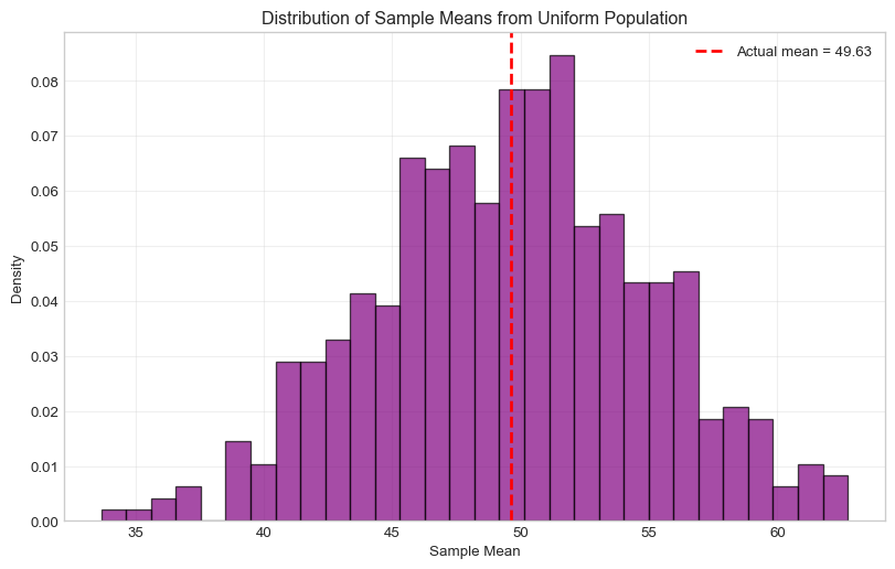
Let’s verify the Central Limit Theorem with a uniform distribution!

# Population: Uniform distribution from 0 to 100 - SOLUTION
population = stats.uniform(loc=0, scale=100)

print("Population (Uniform 0 to 100):")
print(f"Population mean: {population.mean()}")
print(f"Population std: {population.std():.2f}")

# Take 500 samples of size 25 each - SOLUTION
sample_size = 25   # SOLUTION: 25
n_samples = 500    # SOLUTION: 500

sample_means = []
for i in range(n_samples):
    sample = population.rvs(sample_size)  # SOLUTION: sample_size
    sample_means.append(np.mean(sample))

# Check the CLT prediction
predicted_mean = population.mean()
predicted_std = population.std() / np.sqrt(sample_size)

print(f"\nCLT Predictions:")
print(f"Sample means should have mean ≈ {predicted_mean:.2f}")
print(f"Sample means should have std ≈ {predicted_std:.2f}")

print(f"\nActual Results:")
print(f"Sample means actually have mean = {np.mean(sample_means):.2f}")
print(f"Sample means actually have std = {np.std(sample_means):.2f}")

# Make a histogram
plt.figure(figsize=(10, 6))
plt.hist(sample_means, bins=30, density=True, alpha=0.7, color='purple', edgecolor='black')
plt.title('Distribution of Sample Means from Uniform Population')
plt.xlabel('Sample Mean')
plt.ylabel('Density')
plt.axvline(np.mean(sample_means), color='red', linestyle='--', linewidth=2, 
           label=f'Actual mean = {np.mean(sample_means):.2f}')
plt.legend()
plt.grid(True, alpha=0.3)
plt.show()

Population (Uniform 0 to 100):
Population mean: 50.0
Population std: 28.87

CLT Predictions:
Sample means should have mean ≈ 50.00
Sample means should have std ≈ 5.77

Actual Results:
Sample means actually have mean = 49.63
Sample means actually have std = 5.29

Task 4 Solution: Your Own Confidence Interval

Creating a 90% confidence interval for homework time data.

# Homework time data (in hours per week) - SOLUTION
np.random.seed(456)
homework_data = np.random.normal(15, 5, 40)  # 40 students, roughly normal

print("Homework Survey Results:")
print(f"Sample size: {len(homework_data)}")
print(f"Sample mean: {np.mean(homework_data):.2f} hours/week")
print(f"Sample std dev: {np.std(homework_data, ddof=1):.2f} hours/week")

# Create a 90% confidence interval - SOLUTION
# Step 1: Calculate the needed values
sample_mean = np.mean(homework_data)
sample_std = np.std(homework_data, ddof=1)
n = len(homework_data)

# Step 2: Find the critical value for 90% confidence
confidence = 0.90
alpha = 1 - confidence
z_star = stats.norm.ppf(1 - alpha/2)
print(f"Critical value for 90% confidence: {z_star:.3f}")

# Step 3: Calculate standard error and margin of error
standard_error = sample_std / np.sqrt(n)
margin_of_error = z_star * standard_error

print(f"Standard error: {standard_error:.3f}")
print(f"Margin of error: {margin_of_error:.3f}")

# Step 4: Build the confidence interval
ci_lower = sample_mean - margin_of_error
ci_upper = sample_mean + margin_of_error

print(f"\n90% Confidence Interval for average homework time:")
print(f"[{ci_lower:.2f}, {ci_upper:.2f}] hours per week")

# Step 5: Interpret your result
print(f"\nInterpretation:")
print(f"We are 90% confident that the true average homework time")
print(f"for all students is between {ci_lower:.2f} and {ci_upper:.2f} hours per week.")

Homework Survey Results:
Sample size: 40
Sample mean: 15.52 hours/week
Sample std dev: 4.82 hours/week
Critical value for 90% confidence: 1.645
Standard error: 0.763
Margin of error: 1.255

90% Confidence Interval for average homework time:
[14.27, 16.77] hours per week

Interpretation:
We are 90% confident that the true average homework time
for all students is between 14.27 and 16.77 hours per week.

Comparison Questions:

1. How would a 95% confidence interval compare to your 90% interval?
   • A 95% CI would be wider than the 90% CI because we need more “room” to be more confident.
2. What if you had surveyed 100 students instead of 40?
   • The CI would be narrower because larger sample sizes give more precise estimates.

# Demonstrate the comparisons
print("Comparison of different confidence levels:")
print("=" * 45)

# 90% vs 95% confidence intervals
for conf_level in [0.90, 0.95]:
    alpha = 1 - conf_level
    z_crit = stats.norm.ppf(1 - alpha/2)
    margin = z_crit * standard_error
    lower = sample_mean - margin
    upper = sample_mean + margin
    width = upper - lower
    print(f"{conf_level*100:2.0f}% CI: [{lower:.2f}, {upper:.2f}], width = {width:.2f}")

print("\nComparison of different sample sizes (95% CI):")
print("=" * 45)

# Different sample sizes (simulated)
for sample_size_comp in [40, 100]:
    se_comp = sample_std / np.sqrt(sample_size_comp)
    margin_comp = 1.96 * se_comp  # 95% CI
    lower_comp = sample_mean - margin_comp
    upper_comp = sample_mean + margin_comp
    width_comp = upper_comp - lower_comp
    print(f"n={sample_size_comp:3d}: [{lower_comp:.2f}, {upper_comp:.2f}], width = {width_comp:.2f}")

Comparison of different confidence levels:
=============================================
90% CI: [14.27, 16.77], width = 2.51
95% CI: [14.03, 17.01], width = 2.99

Comparison of different sample sizes (95% CI):
=============================================
n= 40: [14.03, 17.01], width = 2.99
n=100: [14.57, 16.47], width = 1.89

Task 5 Solution: Which Distribution Should I Use?

Match each scenario with the best distribution:

# SOLUTION
print("SOLUTIONS:")
print("A. Time between arrivals: 3 (Exponential)")      
print("B. Heights: 1 (Normal)")                    
print("C. Die roll: 4 (Discrete uniform)")                   
print("D. Temperature: 1 (Normal)")                
print("E. Coin flip: 5 (Bernoulli)")                  

print("\nReasoning:")
print("A. Exponential - Time between events follows exponential distribution")
print("B. Normal - Heights of people are naturally normally distributed")  
print("C. Discrete uniform - All 6 outcomes (1,2,3,4,5,6) equally likely")
print("D. Normal - Temperature measurements tend to be normally distributed")
print("E. Bernoulli - Two outcomes (heads/tails) with fixed probability")

SOLUTIONS:
A. Time between arrivals: 3 (Exponential)
B. Heights: 1 (Normal)
C. Die roll: 4 (Discrete uniform)
D. Temperature: 1 (Normal)
E. Coin flip: 5 (Bernoulli)

Reasoning:
A. Exponential - Time between events follows exponential distribution
B. Normal - Heights of people are naturally normally distributed
C. Discrete uniform - All 6 outcomes (1,2,3,4,5,6) equally likely
D. Normal - Temperature measurements tend to be normally distributed
E. Bernoulli - Two outcomes (heads/tails) with fixed probability

🎯 Lab 5 Complete Solutions Summary

• ✅ Task 1: Normal distribution calculations with human heights
• ✅ Task 2: Exponential distribution for bus waiting times
  
• ✅ Task 3: Central Limit Theorem verification with uniform distribution
• ✅ Task 4: 90% confidence interval construction for homework data
• ✅ Task 5: Distribution matching exercise with reasoning

Key Takeaways:

1. Continuous distributions use PDFs and calculate probabilities as areas

2. Normal distribution is fundamental and appears everywhere via CLT

3. Confidence intervals provide ranges of plausible values for parameters

4. Sample size affects precision; confidence level affects interval width

5. Python’s scipy.stats provides powerful tools for distribution analysis